
Matching for Causes without Experiments
Sometimes we have an experiment that we can run to figure out if something is working: give one person a pill and give another a placebo, one person gets a blue button and another gets a green one, one town gets a new health clinic and another doesn’t. Plenty of times though, that just isn’t possible or practical or ethical. Giving someone a blue or green button isn’t likely to change their lives; giving a whole community contaminated drinking water on the other hand, not so trivial. Typically, we (yes, I’m taking some liberties with the we here) as designers aren’t looking to build water treatment plants or change public policy. In service design and complex product design we do often help plan and build things that are complex and that don’t allow for simple experiments. Even more common is finding yourself trying to understand user behavior or assess the value of specific product features without being able to ask users or potential customers survey questions or A/B type queries. In these situations designers and product managers often fall back on mimicking competitors, cursory market research, anecdote, or the old classic design intuition. What if you could dig up some data or collect it yourself and make some informed decisions about a treatment without actually doing the treating yourself? Easier said than done since that data isn’t always easy to come by, but with a little careful poking around and exploring, we can sometimes find ways to look for evidence of causation by looking at treatments of some kind.
Researchers can’t go around risking peoples lives or doing unethical things to understand what effect something might have on a person, a community, an organization. Plenty of other times, we can’t really run an experiment. It’s not practical, it’s not safe, it’s not financially or logistically feasible. But that doesn’t mean that we can’t reason about the causes and relationships of things that we observe. To do this, researchers typically look for “natural experiments”, that is, experiments which are set up by, well, ‘nature’.
Natural experiments vs Observational Studies
Natural experiments are observational studies that can be designed to take advantage of situations that create a treatment group and a control group. This can be any group of entities (people, communities, businesses, et cetera) where selection into treatment or control is random enough that there aren’t clear reasons why a group was picked and where the groups are similar enough that they can be compared. Two neighboring school districts introduce the same new reading program for first grade students. These districts are pretty much identical in terms of demographics, class sizes, teacher experience, and other factors with one key difference: two years ago District A was randomly selected to receive Pre-K funding. We might have a natural experiment that will help us understand the benefits of Pre-K on reading program. That “factors are similar enough” phrase is extremely important. If one school district has classes of 20 and the other classes of 40, you probably shouldn’t compare them directly. If one is much more wealthy than the other, again, probably not an experiment on pre-kindergarten as much as it is an experiment on education and wealth inequality. This is where the concept of matching starts comes in, and it’s extremely important because it’s a way for us to make sure that we have equivalent entities in our ‘treatment’ and ‘control’. If we can be reasonably certain that our entities match across variables but not across treatments then we can start to make educated and informed guesses about what those treatments mean. There are all kinds of natural experiments out there in the world: one state does something while another state does not, an agency runs a lottery, a global pandemic. Now, these tend to be large scale studies that involve many people over large amounts of time.
Lots of studies are just observational studies, that is, they don’t have randomization of some kind. If there’s no randomization, that is, if there’s no treatment that does not closely correlate to a confounding factor, then it’s not really an experiment. As folks interested in causal questions, we want experiments and whenever and wherever we can find them we’re interested because they allow us to be much more certain about causality and effects. There aren’t that many experiments out there though, the more we know about things, the more we realize that randomization is surprisingly difficult to encounter. That doesn’t mean that we can’t reason about causality and effect in these things though, it just means that we have to be more clever in how we do it.
Let’s go back to our two schools and say that one having a pre-K program isn’t accident, it’s got something to do with the funding model of the school or some other reason that we can identify and measure. More on why that last point is important later. Once we think we have a hunch why a school gets a pre-K or not, we can look at the likelihood that they’ll have a pre-K or not, and then look at how that likelihood affects their new reading program, and then how that affects the reading scores that students get on reading tests. There’s a catch here: we People often refer to this as a quasi-experimental design and it’s a fantastic way to work with data that doesn’t have a tidy treat/control divide but that does have distinct characteristics that allow us to measure and separate groups. There’s just one catch: we need more than two schools to do this.
Let’s say that for the sake of writing an interesting article we have a study with 1000 schools in it that includes the average reading scores on some standardized test, whether the school has a pre-K program, whether the school uses a new reading program, and the average class size in the district. Just to be clear: this isn’t an experiment. It’s not randomized between treatment and control. It’s just data. That does not mean however that we cannot do some quasi-experimental analysis. Our data has 1000 row and 4 fields:
scores: an average of the scores on some sort of reading test for a district
reading_program: whether the district has a reading program
pre_k: whether the district has a pre-K program
class_size: the average class size across the district
All of the code for this article lives in this github repository so please check that out if you’d like to run the code and do your own explorations. So, after we do some basic EDA (which we’re going to skip to keep this article a reasonable length) we can do the most basic of estimations of our treatment effects:
mean(dat[dat$reading_program == 1,]$scores) -
  mean(dat[dat$reading_program == 0,]$scores)
Which gives us -0.734 for a treatment effect. So that’s not great if we want our program to increase reading scores. However, we shouldn’t be despondent quite yet. We have, in essence, two treatments. What happens when we look at our score in terms of those two treatments?

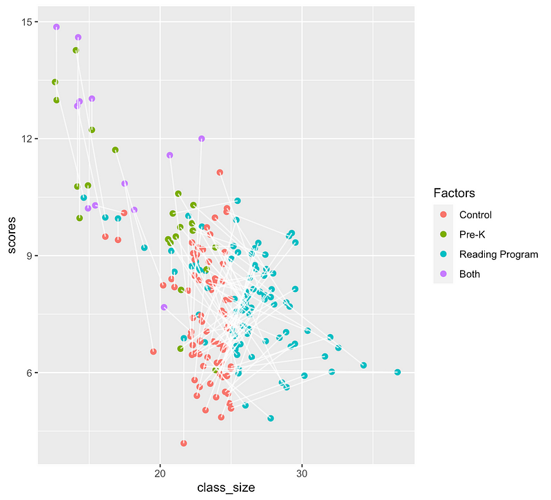
So there’s differences in score, which looks good for our treatments, but also our dataset is very unbalanced: there’s far more control districts than Pre-K or than with a Reading Program and very few with both. What this means, in short, is that we don’t really have an experiment yet. So let’s do some exploratory modeling. We can fit a model using all of our variables:
unmatched <- lm(scores ~ class_size + reading_program + pre_k, data=dat)
summary(unmatched)
This gives us:
Call:
lm(formula = scores ~ class_size + reading_program + pre_k, data = dat)

Residuals:
    Min      1Q  Median      3Q     Max
-5.3989 -1.0350 -0.1092  0.8676 12.2423

Coefficients:
                Estimate Std. Error t value Pr(>|t|)
(Intercept)     15.25750    0.31006   49.21   <2e-16 ***
class_size      -0.34805    0.01435  -24.26   <2e-16 ***
reading_program  1.53241    0.13094   11.70   <2e-16 ***
pre_k            1.60252    0.14072   11.39   <2e-16 ***
---
Signif. codes:  0 ‘***’ 0.001 ‘**’ 0.01 ‘*’ 0.05 ‘.’ 0.1 ‘ ’ 1

Residual standard error: 1.613 on 996 degrees of freedom
Multiple R-squared:  0.639, Adjusted R-squared:  0.6379
F-statistic: 587.6 on 3 and 996 DF,  p-value: < 2.2e-16
There’s things we could do to diagnose the linear regression (normality of errors, distribution of residuals, etc) but there’s something bigger we need to look at first. Our reading program has an effect but so does pre-K and class_size. We want to make sure that our terms are independent of one another. So can class size predict whether a district has a reading program?
# glm formula: predict reading program with class size
predict_reading <- glm(reading_program ~ class_size + pre_k,
                       family="binomial", data = dat)
summary(predict_reading)
We can see that class_size and pre_k do have an effect on having a reading program: the larger the class size, the more likely a district is to have a reading program.
Call:
glm(formula = reading_program ~ class_size + pre_k, family = "binomial",
    data = dat)

Deviance Residuals:
    Min       1Q   Median       3Q      Max
-1.2594  -0.7235  -0.4606   0.5290   3.0087

Coefficients:
            Estimate Std. Error z value Pr(>|z|)
(Intercept) -7.65570    0.59062 -12.962   <2e-16 ***
class_size   0.30409    0.02513  12.101   <2e-16 ***
pre_k        0.65507    0.23597   2.776   0.0055 **
---
Signif. codes:  0 ‘***’ 0.001 ‘**’ 0.01 ‘*’ 0.05 ‘.’ 0.1 ‘ ’ 1

(Dispersion parameter for binomial family taken to be 1)

    Null deviance: 1152.34 on 999  degrees of freedom
Residual deviance:  907.51  on 997  degrees of freedom
AIC: 913.51

Number of Fisher Scoring iterations: 5
We saw that class size negatively affect scores when we don’t account for pre_k but positively affects scores when we do, which means that we have a confounding factor between our treatment (reading_program) and our outcome (scores).
If we graph the influence of each covariate on whether a district has a reading program we can see clear trends for each:

This might be a hint that our reading_program is also being influenced by both class_size and pre_k. Moreover, when we try to see the effect of these covariates on reading_scores we see different results between districts that have a reading program and districts that don’t for the value of the pre_k and the class_size.
Call:
lm(formula = scores ~ class_size + pre_k, data = dat[reading_program ==
    0, ])

Residuals:
    Min      1Q  Median      3Q     Max
-5.4015 -1.0224 -0.0569  0.8961 11.2110

Coefficients:
            Estimate Std. Error t value Pr(>|t|)
(Intercept) 16.94412    0.40289  42.057  < 2e-16 ***
class_size  -0.43261    0.01917 -22.563  < 2e-16 ***
pre_k        1.30763    0.16077   8.133 1.78e-15 ***
---
Signif. codes:  0 ‘***’ 0.001 ‘**’ 0.01 ‘*’ 0.05 ‘.’ 0.1 ‘ ’ 1

Residual standard error: 1.697 on 734 degrees of freedom
Multiple R-squared:  0.6331, Adjusted R-squared:  0.6321
F-statistic: 633.2 on 2 and 734 DF,  p-value: < 2.2e-16
No reading program:
Call:
lm(formula = scores ~ class_size + pre_k, data = dat[reading_program ==
    1, ])

Residuals:
    Min      1Q  Median      3Q     Max
-3.7799 -0.7262 -0.0990  0.6876  3.5185

Coefficients:
            Estimate Std. Error t value Pr(>|t|)
(Intercept) 13.34464    0.47546  28.067   <2e-16 ***
class_size  -0.20956    0.01828 -11.464   <2e-16 ***
pre_k        2.45656    0.27034   9.087   <2e-16 ***
---
Signif. codes:  0 ‘***’ 0.001 ‘**’ 0.01 ‘*’ 0.05 ‘.’ 0.1 ‘ ’ 1

Residual standard error: 1.125 on 260 degrees of freedom
Multiple R-squared:  0.7522, Adjusted R-squared:  0.7503
F-statistic: 394.7 on 2 and 260 DF,  p-value: < 2.2e-16
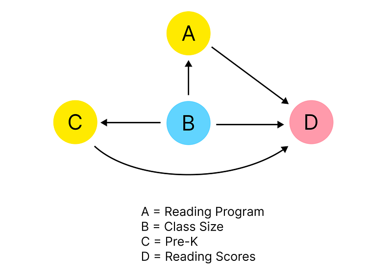
There’s something not quite right here, with a reading program our model estimates quite different influences for pre_k and class_size and gives us a slightly higher r-squared values when we have a reading program than when we don’t. None of these in themselves are problematic but they’re cause for concern. So we can see that our pre-K and our class size are interfering with our reading program in strange ways. Let’s DAG it out and see if we can find out what’s happening
Our Causal Diagram
We want to know how our reading program and the covariates affect the reading scores, but it’s obvious that the existence of a pre-K program affects whether a school has a reading program. Our covariates aren’t a confounder, since we can measure them and control for them but their effect is a selection bias in the treatment.
Obligatory XKCD
This selection bias means that we are seeing the reading program biased by factors that are measurable and have a clear effect. We saw that when we estimated a logistic regression to select for reading_program and found strong evidence that class_size influenced our selection.
Class size is a confounder and a selection bias
What we need to do is to correct the effect that class size is having on our reading program in order to get a better estimate of the reading program itself.
If we have a causal effect we want to estimate but are encountering some confounding variables, we can do our treatment vs control comparison within small groups or pairs where those variables are the same. We’re likely getting an inflated view of the efficacy of our reading program because of how class size is affecting whether a program is in the reading program or not and the reading scores themselves. We’re looking for quasi-experiments and that means that we don’t want selection to overly influence our randomization. What we need is a way to try to find a balance of some kind between the districts with pre-K and reading programs and those without either to understand what each does to the reading scores.
Matching
Matching is a technique which allows us to find close matches across entities in our dataset to perform the kind of comparative modeling that we need to get an accurate assessment of our reading programs effect. There are a few different kinds of matching but in our case we’re interested in Propensity Score Matching (PSM). This is a way of estimating a treatment effect when randomization is not possible and in fact the treatment is being influenced by different variables. The approach comes from the famous paper on PSM written by Paul Rosenbaum and Donald Rubin in 1983. The core of the idea is that you estimate the predicted probability that someone received the treatment based on some explanatory variables. In our case, we know that class size within the districts predict whether a district gets a reading program and that the class size affects the reading score.
So first we want to estimate the likelihood that a district will have a reading program and then estimate the effect of the reading program on the reading score. This is called propensity score estimation and as long as all confounders are included in the propensity score estimation, it reduces bias in observational studies by controlling for variation in treatment that is driven by confounding. In other words, it tries to replicate a randomized control trial by balancing between the control and treatment. Once we have likelihood that a district gets reading program, then we start matching on the other covariates like class size and pre-K. Once we have matched pairs we can estimate the effect that the reading program have on reading scores by looking at the differences between our pairs. When we have a clear picture of how two districts are the same, we can start to build a more clear picture of how they might be different as well and we remove the
First, we need to match. We’re going to use the matchit library to find pairs in our data.
match <- matchit(reading_program ~ class_size + pre_k,
                 data = dat, method = "nearest", distance = "glm")
summary(match)
We set the formula to select what we’re matching on. We want pairs of schools on either side of the pre-K selection with class sizes that are as close as possible. Calling summary() gives us the results of our matching:
Call:
matchit(formula = reading_program ~ class_size + pre_k, data = dat,
    method = "optimal", distance = "glm")

Summary of Balance for All Data:
           Means Treated Means Control Std. Mean Diff. Var. Ratio eCDF Mean eCDF Max
distance          0.4636        0.1914          1.0112     3.9514    0.2846   0.5964
class_size       23.8223       18.5544          0.9440     1.8445    0.2860   0.6008
pre_k             0.1711        0.3989         -0.6049          .    0.2278   0.2278

Summary of Balance for Matched Data:
           Means Treated Means Control Std. Mean Diff. Var. Ratio eCDF Mean eCDF Max Std. Pair Dist.
distance          0.4636        0.3067          0.5829     3.5817    0.1032   0.5817          0.5835
class_size       23.8223       21.1680          0.4756     2.3211    0.1139   0.6008          0.5173
pre_k             0.1711        0.3346         -0.4341          .    0.1635   0.1635          0.7370

Sample Sizes:
          Control Treated
All           737     263
Matched       263     263
Unmatched     474       0
Discarded       0       0
So we can see that our new data set removes about 68% of our records but also balances the treatment and the control far better. The Std. Mean Diff column shows how different the means for each variable are in the matched and unmatched data sets. We also now have balance between our controls and our treatments: 234 in each. The generally accepted term is matching but the pruning aspect of matching is just as important because a better matched dataset will provide better estimates. This is important because regression likes high variance features, that is, it will generally over-emphasize the effect of features that have high variance and any non-normality. Balancing our dataset gives us a better shot at getting OLS regression to do estimate our effects more accurately.
Let’s look at the matching:
There are clear biases here with regard to class size, pre-K, and our reading program, but matching across reading program status can help control for that. Now that we have a matched dataset, we can use it in a linear regression:
#build our matches into a usable dataset
match_data = match.data(match)

#run the regression on our dataset with an interaction formula
lm_matched =lm(scores ~ class_size + reading_program + pre_k, data=match_data)
summary(lm_matched)

Now we can look at our regression output and see whether it might be different than what we originally saw:

Call:
lm(formula = scores ~ class_size + reading_program + pre_k, data = match_data)

Residuals:
    Min      1Q  Median      3Q     Max
-3.9577 -0.8770 -0.0892  0.7923  4.9938

Coefficients:
                Estimate Std. Error t value Pr(>|t|)
(Intercept)     12.77163    0.37716   33.86   <2e-16 ***
class_size      -0.23520    0.01557  -15.11   <2e-16 ***
reading_program  1.22803    0.11826   10.38   <2e-16 ***
pre_k            2.19827    0.17179   12.80   <2e-16 ***
---
Signif. codes:  0 ‘***’ 0.001 ‘**’ 0.01 ‘*’ 0.05 ‘.’ 0.1 ‘ ’ 1

Residual standard error: 1.305 on 522 degrees of freedom
Multiple R-squared:  0.6702, Adjusted R-squared:  0.6683
F-statistic: 353.5 on 3 and 522 DF,  p-value: < 2.2e-16
Here we’re see an effect for our reading program that we can have a little more confidence in. Our adjusted R-squared is a little bit higher (0.67 vs 0.62) and our residual standard error is lower (1.3 vs 1.6).
So now that we’re accounting properly for how the class size influences whether a district has a reading program and how a pre-K and how the class size influence whether they get a reading program. The interaction terms are a bit confusing though because they show a separate increase for reading_program_factor and pre_k_factor but a decrease for the two of them. That’s because with our balanced dataset we’re trying to account for each individually but cumulatively, they don’t equal a 11.1 increase in reading_score. To make this clearer, we can use the marginaleffects package to get values for the individual features:
library(marginaleffects)

#use our model, calculate for our variables that contribute to reading_score:
summary(comparisons(lm_matched,
                    vcov = ~subclass,
                    variables = c("reading_program", "pre_k")))

This gives us a cleaner comparison of each feature:

 Term Contrast Effect Std. Error z value   Pr(>|z|)  2.5 % 97.5 %
1 reading_program    1 - 0  1.228     0.1169   10.50 < 2.22e-16 0.9989  1.457
2           pre_k    1 - 0  2.198     0.1845   11.92 < 2.22e-16 1.8367  2.560
That’s different than our original model, which over-estimates the effect of the reading program and under estimates the effect of pre-K:
 Term Contrast Effect Std. Error z value   Pr(>|z|) 2.5 % 97.5 %
1 reading_program    1 - 0  1.532     0.1309   11.70 < 2.22e-16 1.276  1.789
2           pre_k    1 - 0  1.603     0.1407   11.39 < 2.22e-16 1.327  1.878
So our matching both gives us a more accurate estimate of the effect and a model with a higher r squared and lower standard errors.
We can then predict how our factors, pre_k, reading_program, and affect the reading_score with a call to marginal effects predictions():
# get some predictions for each reading_program, pre_k value, and for the max
# and min of the class_size
p <- predictions(
  lm_matched,
  variables = list(reading_program = c(0,1)),
  newdata = datagrid(pre_k = unique, class_size = range))
So we can see how each of the variables interact:
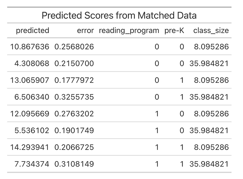

Unsurprisingly, the districts with small class sizes and either pre-K or reading programs perform best (note the errors between the 3 variants). Notice that the errors for the matched data are higher with the class size is higher and lower when the class size is lower but generally about the same or slightly lower than our unmatched data predictions. We now have strong evidence that our reading program is effective and that the matched data helped us better estimate the effect of the reading program and the other covariates. Matching isn’t always the solution to quasi-experimental design, in fact, many time it isn’t a valid option, but when you have confounders and imbalanced data, it can create a more meaningful dataset with better opportunities for causal inference.
What’s this got to do with design?
So what does all of this tell us? Well, we couldn’t run an experiment. We didn’t have random selection at all and we had a confounders that made measurement extremely difficult. But we also were able to get solid results from a quasi-experimental set up by matching our districts by how likely they were to have a reading program and then comparing them by their performance with and without that program. So we can still use experimental methods when we can’t run experiments as long as we’re thoughtful about how we do the measurement. Matching can help us estimate causal effects of a treatment or exposure on an outcome while controlling for measured pre-treatment variables. In our case the income and spend variables confounded our measurements, but we could still control for that.
Now to the why for design of services, websites, programs, public policy: this makes treatments that’s aren’t random still usable as treatments and thus data that isn’t truly experimental useful for evaluating causal effects. There are so many times that we can’t run an experiment but we do have data that shows an exposure or a treatment. To throw our hands up any time that we’re confronted with that kind of data would be a waste of an opportunity to learn about our users, our designs, or our business. Tragic! Instead of giving up, we should see if we can match and then assess. Many times matching won’t work but many times it will and in these times it can be a powerful tool for understanding how we can make causal inferences even in those situations. This becomes particularly important when we’re dealing with information from services or multi-step processes. You can’t just A/B all of something complex, you have to do a single part of it, but then what leads up to that part frequently becomes a part of your analysis whether you want it to or not. Even if you’re not running the analysis, designing the ability to collect data into your system or service makes the work of whatever organization or entity that you’re with easier and better. Those can be surveys, key points for interviews, specific moments to capture in telemetry, or even topics to probe with users in usability studies.