
I wrote a few articles last year that explored how we could look at how measuring what a redesign of a service caused. In a hypothetical customer service scenario, the hypothesis that a redesign might cause people to give the service a higher rating or to quit using it less was explored using Latent Class Analysis. One comment that my friend Francesca Desmarais made when reviewing that article for me was that the sample size was massive. What would the article look like with a way smaller sample size? 1000 respondents is totally reasonable A/B test size for a large popular website. With a sample size like that your statistical power will be through the roof. However in the world of the design research, social sciences, or public health, one is far more likely to encounter far smaller sample sizes, think 30 to 40 respondents. Working with small studies like this means that the confidence intervals we can assume to be reasonably small in larger studies will be worryingly large. In other words, if you think a two degree rise in temperature leads to a roughly $2 increase in the amount that someone will pay for ice cream, an experiment with a large sample size might let you say that you’re 95% confident that it’s between $1.90 and $2.10, a small sample size might leave you forced to admit that you’re 95% confident that it’s somewhere between -2.00 and +4.00. That’s not the kind of confidence-inspiring math that the ice cream magnates of the world want to hear.
Just because we have to deal with uncertainty though doesn’t mean that we can’t deal with it well, it just means that we have to be smart about how we’re doing it. There’s two fundamentally different approaches to doing statistics and while the scope of laying out how they are different is way way way beyond the scope of this article, looking at how those two approaches are similar and different when dealing with really small samples is not actually that hard if you ignore a lot of the philosophical differences and focus on what you get out of each method. In this article I, and by extension you, are going to be totally methodology-agnostic and application-focused statisticians with zero interest in academic and philosophical battles. What we’re interested in is whether it helps us understand the whether there is a treatment effect and get a sense of the size of that treatment effect.
The first of our two approaches is the frequentist approach which says (warning: extreme simplification) that we should run experiments or trials and each of those is completely independent of any other experiment or trial. The second approach is the Bayesian approach, which says that you can (and should) use information or beliefs from previous trials to help inform your understanding of current experiments and trials. Which is better? Both. Any trained statistician reading this may be dismayed that I’m going to leave it at that but we’ve got an experiment to analyze.
The Experiment
So let’s look at our small sample size experiment: we have a new way of teaching multiplication to 9 year olds and we want to see how well it does across a few different classrooms. We run a randomized trial using a few different classrooms and test their grades on a test before and after treatment. Here’s our data:
We have a way of looking at how kids do before the experiment and after the experiment, which is some sort of test score encoded here as prev_grade and post_grade. Now, this is only 20 records and the kids are spread out across 4 different classrooms, this is certainly not the ideal scenario but it’s also something that we can work with if we’re willing to accept the uncertainty that comes with working with smaller sample sizes. The code for this article will all be written in R and the R files to run it all live in this github repository.
First things first, we want to load our file and create a field that will allow us to see how much the grades change in our treatment and control group:
experiment <- read.csv(“data/simple_experiment_small_2.csv”)
experiment$grade_diff <- experiment$post_grade — experiment$prev_grade
Now that we’ve got our data, the first thing we’ll want to do is to determine whether there is a different between our treated group and untreated group, so we create a grade_diff variable.
In a frequentist approach, we’ll compare our treatment and control groups with a t-test:
t.test(experiment[experiment$treated == 1,]$grade_diff,
  experiment[experiment$treated == 0,]$grade_diff)
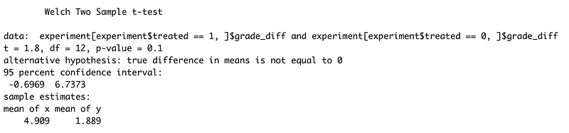
Frequentists use p-values, essentially the likelihood that if the two groups would appear to be different even if they were the same. Here we have a p-value of 0.1, which is ok but isn’t fantastic. Usually frequentists look for a p-value of 0.05 or under by convention (which is silly honestly but whatever) though we can see that the 95% confidence interval includes a great deal of difference (a lowest value of -0.69 and a highest value of 6.73). So we’re not off to the greatest start because our treatment can’t be established to be effective. Now let’s take a look at the Bayesian approach to exploring the difference of our two groups:
ttestBF(experiment[experiment$treated == 1,]$grade_diff,
  experiment[experiment$treated == 0,]$grade_diff)

That’s not spectacular either. The Bayes Factor is quite similar to a p-value in how we use it (establishing whether the two groups are similar or not) but is conceptually quite different because it’s actually a measure of how likely one hypothesis is (these groups are different) over the other hypothesis (these groups are the same).

So our 0.97 is in the ‘no evidence’ range. So far, we don’t seem to have a real treatment effect but let’s look a little more closely.
Our treatment variable thus far has been treated as if it’s a numeric variable and that’s not quite true. Instead of treating it like a numeric value which happens to have two different values, we should treat it like a factor which has two different categories: kids in the treatment group and kids not in the treatment group. We should do the same with our classroom: classrooms aren’t a numeric value really, they’re just an indicator of which classroom the kid is in. So we want both variables to be factors:
experiment$classfactor <- factor(experiment$classroom)
experiment$treatedfactor <- factor(experiment$treated)
Now we can start to evaluate whether our treatment or classroom or a combination of the two can help us uncover a treatment effect or confirm that there is no treatment effect whatsoever.
We’re going to make heavy use of formulas to describe the relationships between our variables which are going to look like this:
- A dependent variable we want to predict.
- A “~”, that we use to indicate that we now give the other variables of interest. (comparable to the ‘=’ of the regression equation).
- The different independent variables separated by the summation symbol ‘+’.
So if we want to predict grade_diff and we think it’s affected by our treatedfactor we use the following formula:
grade_diff ~ treatedfactor
If we want to predict grade_diff and we think it’s affected by our treatedfactor and our classroomfactor, we use the following formula:
grade_diff ~ treatedfactor + classroomfactor
Again we begin first with the frequentist approach and a very naive model:
f_aov <- aov(grade_diff ~ treatedfactor, data = experiment)
summary(f_aov)

That’s not especially different than the t-test value that we established earlier, around 0.12, moreover, the F value isn’t great either. The F statistic is a ratio of 2 different measure of variance for each field in the data. If the null hypothesis is true then the factors are all estimating equivalent entities and the ratio will be around 1. Since the F value of our treatment is 2.62 , we aren’t quite certain that our values are distinct enough to have correctly calculated coefficients in a linear regression for the treatment. We can’t say that our treated factor lets us understand much about the effect that treatment has on our grade difference. What if we bring our classroom factor into this?
f_aov <- aov(grade_diff ~ treatedfactor + classfactor, data = experiment)
summary(f_aov)
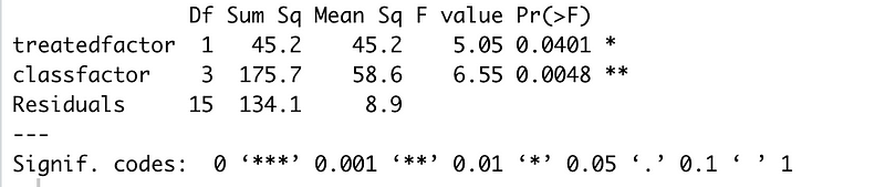
Now this is starting to look more promising: our treated factor has a p-value of 0.04 and the F-value for treatment and classroom are much higher. But what about how the classroom affects the treatment itself? Is that important? Checking the analysis of variances for the interactions of classroom and treatment will give us a better picture of whether treatment and classroom interact.
f_aov <- aov(grade_diff ~ treatedfactor:classfactor, data = experiment)
summary(f_aov)
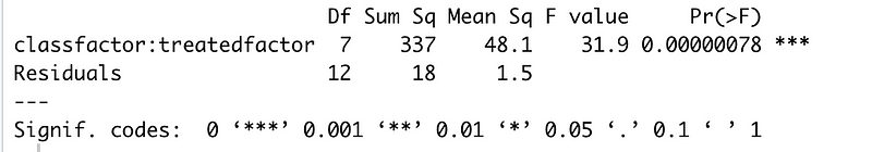
Bingo! That’s a very very low p-value and a strong F value and what that tells us is that there are real differences between classrooms for the treatment. Accounting for those interactions will give us a clearer picture (even with our tiny sample size) of what effect our treatment might have in different classrooms.
Now let’s do the Bayesian approach to this with anovaBF. What we want to know first is which combination of our variables will be useful in building our model:
anovaBF(grade_diff ~ treatedfactor * classfactor, data = experiment)

We can interpret the Bayes Factor here in the same way as the Bayes Factor for the t-test. There’s no evidence that the treatedfactor model is any different from an intercept only model and good evidence that a classroom is better. A classroom and treatment model has strong evidence to be a better fit than an intercept alone model, whereas a model with treatment and classroom interactions has ridiculously strong evidence.¹
Modeling
Now that we have a picture of what our model should look like in a Bayesian context, let’s look at creating and evaluating the model itself. The Frequentist approach to fit a linear regression is to pass the dataframe (in our case we’ve called it experiment) to the lm() function with a formula:
flm <- lm(grade_diff ~ treatedfactor * classfactor, data = experiment)
This asks R to fit each coefficient using a process called Ordinary Least Squares, more commonly known as OLS. OLS looks to minimize the sum of square differences between the observed and predicted values, so that the predicted values of the coefficients most closely match the values we see in the data. Think of this process as fitting a line that generally describes all of our records with an intercept and multiple coefficients that can pull an individual record a little in one direction or the other. The goal is that we should be able to use our model to predict the likely output for a given input. In our case that would be a previous grade, what classroom they’re in, and whether they got the treatment or not. Now let’s check out what our linear regression output looks like by using stargazer:
stargazer::stargazer(flm)
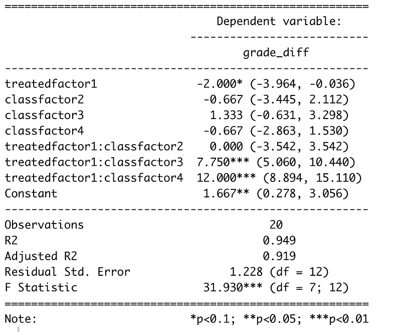
What we see here is the coefficient values for individual factors like treatedfactor1 which is whether a student gets the treatment or not, and interaction terms like treatedfactor1:classfactor3 which is a student who has gotten the treatment and is in classroom 3. We’re in a frequentist context here, so we want to ignore pretty much anything that has a p-value higher than 0.05 as being inconclusive, which is unfortunate because quite a few of our coefficients aren’t conclusive. That’s the pain of working with small datasets. However, we can draw a few conclusions from this. We can see is that the overall treatment is not conclusively effective throughout the classrooms but that it does seems to be effective in some of the classrooms. In Classroom 1 and 2, it doesn’t seem to make much of a difference while in Classrooms 3 and 4, our treatment has a large effect. For Classroom 4 the estimated treatment effect would, on average, be ²
Intercept + treated + classfactor4 + (treated*classfactor4)
or
1.667 - 2 - 0.667 + 12 = 11
So seems as though the variation in our classrooms was masking the treatment effect. Separating the different classrooms, even though some of the classrooms had as few as 3 students represented, helped us get a better measure of the treatment effect. Another statistic that we can look at is the adjusted R-squared, which will help us understand the amount of variation in the data that is explained by the model. In this case the adjusted R-squared estimates that 94.9% of the variation in the model is explained by our treated and classroom factors. Now, we still have a larger problem that our treatment doesn’t have a clear output independent of classrooms and that’s not great for our calculation of an overall treatment effect but we’ll come to that in the next section of this article.
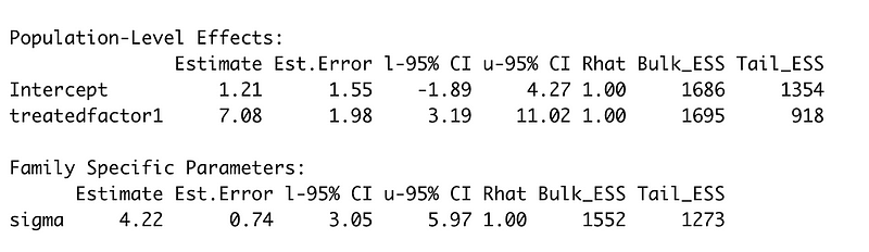
Now we should look at the Bayesian approach to the same model. Instead of using lm(), we use brm() but much of the rest of the call should look familiar to you:
bayes_lr <- brm(grade_diff ~ treatedfactor * classfactor,
  data = experiment,
  refresh = 0,
  warmup = 500,
  iter = 1000)


# print our results
summary(bayes_lr)

Quite similar results to our frequentist approach above, though with a dramatically different way of arriving there. Let’s look at how they’re similar:
- The treatment isn’t especially significant and seems to be negative. We don’t get p-values because we’re looking at the probability that distributions match evidence but our confidence intervals are quite wide (-4.4 to 0.42)
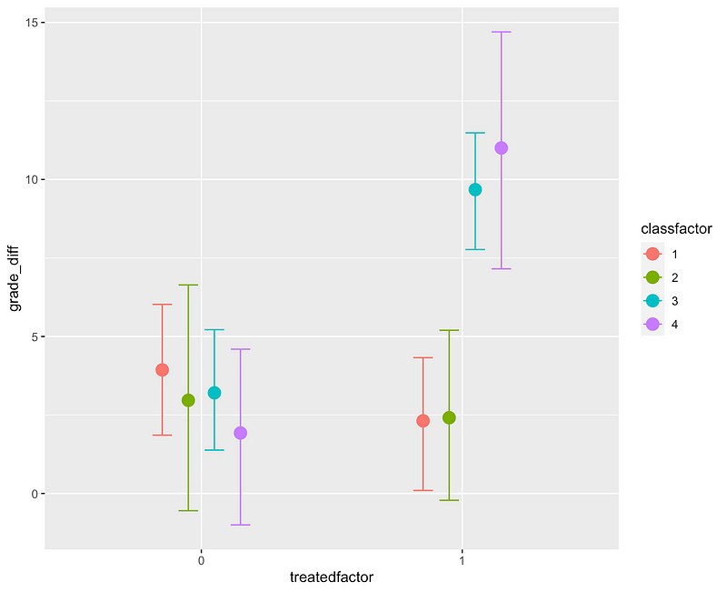
- Being in classrooms 1 or 2 and being treated has no effect.
- Being treated in classrooms 3 and 4 does have an effect (increase of 7.77 and 12.09 with errors of 1.59 and 1.9)
We can double check the importance of our interaction effects with a call to conditional_effects()
We’ll come back to what’s going on between our classrooms in a moment. First: what’s going on under the hood in the Bayesian context that’s different from the frequentist context? Well, this is a very big topic that I’m about to brutally reduce but brm runs our model many times (1000 times in our case) with slightly different values for each coefficient and assesses how the output distribution fits the data. In essence, we try some values for each coefficient and see how likely it is that that the distribution generated by that combination of coefficients would match the actual data that we see. When the algorithm lands on a perfect fit of the posterior distribution, or as good of a fit it can find given the size of our dataset, we stop picking new coefficients and give the result. Here’s a better and much longer description. Now, there’s a big part of the Bayes theorem that’s missing here and that’s the prior. We didn’t pick a prior, we just let brm pick one for us and we still landed in a pretty reasonable place. That’s slightly frowned upon in the Bayes world but we’re pretending we know nothing about our classrooms or our treatment. So wait, you may be thinking, what if we did know something about them?
What’s up with the Classrooms?
Back to our classrooms, though. Can we say that we have a population wide causal effect? No, we can’t prove that. Can we say that classrooms cause higher test scores but only with the new teaching methods? Again, no, and that doesn’t really make much sense. Is there something that we should be measuring that we didn’t?This is where the detective work of causal inference comes in, so we go dig a little deeper.
Looking at our conditional_effects() graph above, it’s obvious that there’s no effect in Classrooms 1 and 2 and that’s just, well, interesting. Let’s go back to the moment before we started fitting our model and imagine that we’re puzzling over our data and a colleague who has worked in the same school just happens to walk by. “Oh, did you know that Classrooms 1 and 2 already did the fancy new multiplication teaching method last semester?”³ they ask. Palm to forehead you explain that you did not. That explains why the classroom interactions were so important though. Experiment ruined? Well, not necessarily. What we just heard is that we don’t have population level effects (aka “fixed effects”). Our effects are all group level effects (aka “random effects”), which is to say that we do have a treatment effect but that it’s at the level of which classroom a student is in, rather than something that exists across all classrooms.⁴ So we now have two approaches: use our information to create a posterior or create a model that models those group effects. Bayes Theorem says: your posterior (e.g. outcome) is equal to the likelihood times your prior divided by your marginalization. We were just letting brm pick a prior for us previously. Our colleague just happened to give us a pretty reasonable prior and that prior says: the distributions for Classrooms 1 and 2 with the treatment are probably going to be zero because they’ve already done the treatment and the treatments for Classrooms 3 and 4 are probably significant. Let’s incorporate that into our model fitting:
# priors for our interactions
prior_strong <- c(
  prior(normal(0.0, 2.0), coef = treatedfactor1:classfactor1), # no effect
  prior(normal(0.0, 2.0), coef = treatedfactor1:classfactor2), # no effect
  prior(normal(6.0, 2.0), coef = treatedfactor1:classfactor3), # effect
  prior(normal(6.0, 2.0), coef = treatedfactor1:classfactor4)  # effect
)

#Bayes:  using our prior
brms_strong_prior <- brm(grade_diff ~ treatedfactor : classfactor,
                      prior = prior_strong,
                      data = experiment,
                      refresh = 0, warmup = 500, iter = 1000)


summary(brms_strong_prior)
We say that our priors for treatedfactor1:classfactor1 and treatedfactor1:classfactor2 are a normal distribution centered around 0, and that classrooms 3 and 4 maybe are a normal distribution centered around 6. We then acknowledge that there is no overall treatment effect by changing grade_diff ~ treatedfactor * classfactor to grade_diff ~ treatedfactor : classfactor.

Now we get smaller estimates for our Classroom 3 and 4 treatments but a near 0 estimate for our treatment and for the effect of treatment on Classrooms 1 and 2. Sounds more like what our colleague just explained to us.
Now, these are still population level effects and that shouldn’t seem quite right. We can specify group level effects with a slightly different syntax:
#Bayes: group level effects
bayes_group <- brm(
    grade_diff ~ (treatedfactor | classfactor),
    data = experiment,
    refresh = 0,
    warmup = 500,
    iter = 1000,
    control=list(adapt_delta=0.95)
    )

# get our group level effects (aka 'random effects')
ranef(bayes_group)

Read this as the treatment effect for each classroom. So treatment in Classroom 1 indicates possibly a reduction of -2 in score whereas treatment in Classroom 4 indicates an increase of 8.8 in score. Not remarkably dissimilar from what we saw with our priors.
Now, the flip side of this is the frequentist approach, which is a little more complicated when our colleague walks over. Frequentists don’t have the same concept of “priors” or random effects so we can’t just pop our estimate of them into our linear regression in the same way. A strict frequentist would need to re-run the test with a new method of some kind, find a new set of classrooms, or integrate the data from the previous multiplication teaching method.
But, to make things easy on ourselves, let’s say that our colleague just happens to have the data from that previous multiplication teaching experiment and is willing to provide it. For our frequentist approach we can just merge our previous data and our new data (after checking that we can in fact run a linear regression).
prev_data <- read.csv("data/experiment_update.csv")

#make it match our experiment
prev_data$grade_diff <- prev_data$post_grade - prev_data$prev_grade
prev_data$classfactor <- factor(prev_data$classroom)
prev_data$treatedfactor <- factor(prev_data$treated)

# merge the two but toss class 1 and 2 from OUR experiment
merged <- merge(
    experiment[experiment$classroom > 2,],
    prev_data,
    all = TRUE
    )

# now rereun with our new data
merged_model <- lm(
    grade_diff ~ treatedfactor*classfactor,
    data = merged
)
stargazer::stargazer(merged_model)
This gives us back the following:

So now none of our interactions have a meaningful value any more but our treatment does have a very strong value. Simplifying the model gives us a much better view of our treatment effect using our merged data:
# now rereun with our new data
simple_merged_model <- lm(grade_diff ~ treatedfactor, data = merged)
stargazer::stargazer(simple_merged_model)

The R-squared isn’t amazing here because we’re missing all of our classroom level effects, which we know exist, but we have an accurate picture of the treatment. What about the Bayesian approach to using our previous data? Well, we could run a regression on our previous data and use it as a prior for our more recent data:
bayes_lr_previous <- brm(grade_diff ~ treatedfactor,
                          data = prev_data, refresh = 0,
                          warmup = 500, iter = 1000)
summary(bayes_lr_previous)
The treatment factor seems credible. This is where we can do some critical thinking and think that since we now have accurate information about the treatment across all of our classrooms but they’re not represented correctly, we can fix some of that with our priors. So let’s take our treatment factor for our classrooms as a prior and redo our model:
# priors from grade_diff ~ treatedfactor
# for only classes 1 and 2

brms_prior <- c(
  prior(normal(7.0, 0.5), coef = treatedfactor1)
)

bayes_lr_prior <- brm(grade_diff ~ treatedfactor,
    prior = brms_prior,
    data = experiment,
    refresh = 0,
    warmup = 500,
    iter = 1000
)

summary(bayes_lr_prior)

This brings us close to what we got for our frequentist linear regression above and simplifies our Bayesian model. Job done? Well there’s one last question: is it as good as our group level random effects model? We can test models using loo_compare
#check group vs smaller priors
loo_compare(loo(bayes_lr_prior),
loo(bayes_group))
#group is much better

#check group vs larger priors
loo_compare(loo(brms_strong_prior), loo(bayes_group))
#group is slightly better
So, our group level formula out-performs either of our prior based models, which isn’t always the case in small studies, but then we compared multiple different methods and can develop our analysis further depending on how much we trust the previous study or its results.
Wrap Up (Finally)
So what did we learn? Earlier we could have said that classroom and treatment affect test scores but there’s a common sense part of causal analysis that we need to take into account here: we can’t just “do the math”. We need to do some reasoning about it as well. The classroom really shouldn’t affect our treatment as much as it seems to. Controlling for the classroom (and getting some updated data) allows us to get an estimate for a treatment effect in our experiment dependent on those classrooms. We can say with some confidence that our treatment has an effect of between 5.8 and 7.7 points on math test scores, even with studies of only 20 or 31 samples. As designers thinking about usability tests or small pilot studies, realistically we can imagine studies that are about this size. It’s important to think what a linear regression can tell us (“is there a treatment effect?”) and what it can’t (“why are different groups affected differently by the treatment?”). Working with small datasets sometimes requires that we design our research around our design questions in careful ways and requires us to be very clever about how we analyze that data. If you can think of other topics in quantitative research and design that you’d like to dive in with me, please leave a suggestion. Thanks!
Footnotes
[1] I find this sort of Bayes Factor analysis to be a little more helpful than comparing Adjusted R-squared values since they are the result of a direct comparison between two models but the overall effect is more or less the same: we can see how well different types of models might fit our data.
[2] Note that this isn’t a guarantee that a student in classroom 4 receiving our new treatment will have a grade difference of +11, it’s that on average students in classroom 4 who receive our new treatment, will show a grade difference of +11.
[3] You may notice that our effective sample size just shrank even further from 20 to 11, can we still do anything with that?
[4] The ‘random effects’ and ‘fixed effects’ nomenclature is confusing because it means different things with different kinds of data and because statisticians aren’t as interested in being precise with language as they are with data and modeling.