Do you like predicting the future? Of course you do. You'll be a billionaire, you'll save the planet, you'll wait until just the right moment to buy that plane ticket, the list goes on. Of course, actually predicting the future is a bit more boring than that. Most of the time we want to predict things like when machine on a production line might start failing or when there might be a spike in demand for electricity. We call this kind of prediction "forecasting" and while it does predict the future, a far better way of thinking about it is that it carefully examines the past for patterns and projects those into the future. This means that your past data, the time series data which represents the past of the thing you're trying to predict, is vitally important. Poor historical data = poor future predictions. Good historical data = good future predictions.
Forecasting and Bigger is Better?
Transformers definitely are not the only way to do time series forecasting, but they are a really interesting way to approach it. You're almost certainly familiar with Transformers from NLP applications and there the name of the game almost always is "bigger". Bigger means better and better means more generative ability, better translations, better summarization. Here's a question though: is it the same in long-term time series forecasting? I've always been curious about this as I once spent a lot of time working on forecasting eviction rates and our approach in that project was to work with an NBEATS architecture
Recently though I came across a fascinating paper that raised some interesting questions about the efficacy of transformers for forecasting:
...in time series modeling, we are to extract the temporal relations in an ordered set of continuous points. While employing positional encoding and using tokens to embed sub-series in Transformers facilitate preserving some ordering information, the nature of the permutation-invariant self-attention mechanism inevitably results in temporal information loss
Put a little more pointedly:
...we pose the following intriguing question: Are Transformers really effective for long-term time series forecasting?
They tested against several SOTA transformer architectures: FEDformer, Autoformer, Informer, Pyraformer, and LogTrans and found that what they describe as "a set of embarrassingly simple one-layer linear models named LTSF-Linear" outperforms many of these architectures on canonical time series datasets. Their paper is excellent and I'd highly encourage you to give it a skim. This feels to me like a wonderful question to probe a bit on: with a complex dataset which has multiple covariates and multiple locations.
So first, our dataset: the Beijing Air Quality dataset
This dataset is usually used to teach data science students about regression tasks or to help compare tree and regression models to predict PM2.5 quality based on other characteristics but we're going to try to use it to forecast, which is a more complex task. We'll pick a few models and a toolkit that makes it easy to compare and train them. The toolkit: DARTS. The models: Temporal Convolutional Network, Temporal Fusion Transformer, NBEATS, NHiTS, DLinear (from the above paper), and of course a Naive Drift Model for baseline comparison.
First, we want to train all our models. The way that DARTs sets up configuring the properties of the models, it can be a little bit difficult to understand what the best parameters might be since there's not a direct correlation between properties of the dataset and the best settings for the model itself. I'll admit that what I chose were a little haphazard, selecting three or four permutations, training, then testing. I burned through my Google Colab credits pretty quickly. I'll admit that there likely may be slightly better performing versions of these models but that the general gist of them should be accurate enough. On to the testing.
The goal
Our models should be able to forecast PM2.5 for a given station using historical time series data, past covariates, and future covariates if the model supports that.
The data
We have hourly readings from 6 different sites in the Beijing area. The fact that this dataset contains multiple different time series makes it a bit more complex and challenging than a typical time series dataset. First off, we should look to see what our timeseries data looks like, whether it's seasonal and stationary, and then we can look to see what these different stations mean for us:
To keep this blogpost from being an absolute wall of code, I'm going to just point to specific parts of the notebook files in places and instead discuss the results.
First, we want to turn our data into properly timestamped data with stations and wind direction as indices rather than strings:
| index | year | month | day | hour | PM2.5 | PM10 | SO2 | NO2 | CO | O3 | TEMP | PRES | DEWP | RAIN | wd | WSPM | station | timestamp |
|---|---|---|---|---|---|---|---|---|---|---|---|---|---|---|---|---|---|---|
| 0 | 2013 | 3 | 1 | 0 | 4.0 | 4.0 | 4.0 | 7.0 | 300.0 | 77.0 | -0.7 | 1023.0 | -18.8 | 0.0 | 0.0 | 4.4 | 0 | 2013-03-01 00:00:00 |
| 1 | 2013 | 3 | 1 | 1 | 8.0 | 8.0 | 4.0 | 7.0 | 300.0 | 77.0 | -1.1 | 1023.2 | -18.2 | 0.0 | 1.0 | 4.7 | 0 | 2013-03-01 01:00:00 |
| 2 | 2013 | 3 | 1 | 2 | 7.0 | 7.0 | 5.0 | 10.0 | 300.0 | 73.0 | -1.1 | 1023.5 | -18.2 | 0.0 | 0.0 | 5.6 | 0 | 2013-03-01 02:00:00 |
| 3 | 2013 | 3 | 1 | 3 | 6.0 | 6.0 | 11.0 | 11.0 | 300.0 | 72.0 | -1.4 | 1024.5 | -19.4 | 0.0 | 2.0 | 3.1 | 0 | 2013-03-01 03:00:00 |
| 4 | 2013 | 3 | 1 | 4 | 3.0 | 3.0 | 12.0 | 12.0 | 300.0 | 72.0 | -2.0 | 1025.2 | -19.5 | 0.0 | 1.0 | 2.0 | 0 | 2013-03-01 04:00:00 |
First things first with a time series, we need to check that it's stationary and non-seasonal. First up, an empirical visual inspection:
Monthly:
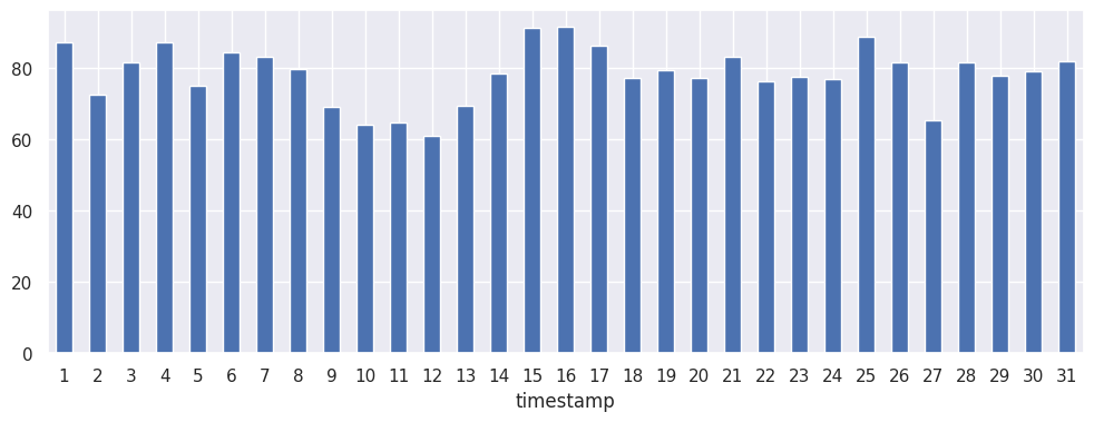
Hourly:
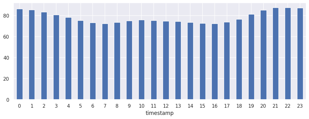
Patterns present but nothing that indicates seasonality that we need to worry about. Running seasonal_decompose gives us the following:
max : 10.28236607142857
min : -8.78365956959707
mean : 7.218984415827502e-17
We also check that this is stationary with a KPSS and ADF test (yay, good old fashioned stats!) Stationarity
Next, we can use the SelectKBest to look at what affects PM2.5 SelectKBest
Feature 2 CO: 550607.964325
Feature 1 NO2: 318532.401779
Feature 0 SO2: 122550.324105
Feature 5 WSPM: 29596.179859
Feature 3 O3: 8753.722415
Feature 4 TEMP: 7466.488882
Feature 6 wd: 3120.139781
Feature 7 station: 428.761398
CO is strongly predictive of PM2.5 and stations are not. But let's think a bit about this: we could guess that air pollution in one part of the city might be worse than others. It could be tempting to flatten everything down to remove the distinctions of the stations but we should also make sure that our stations aren't significant when treated like a time series. One way of doing this is to use Dynamic Time Warping to see how different our time series are from one another.
What we want from dynamic time warping is a metric of how much we would need to move one single valued time series in order to make it match another. In this case, a Euclidean distance is simple and easily interpretable:
dist_mat = pd.DataFrame()

for i in df['station'].unique():
  dist_station = []
  x = np.array(df[df['station'] == i]["PM2.5"])
  for j in df['station'].unique():
    if(i != j):
      y = np.array(df[df['station'] == j]["PM2.5"])
      dtw_distance, warp_path = fastdtw(x, y, dist=2)
      dist_station.append(dtw_distance/len(x))
    else:
      dist_station.append(-1)

  dist_mat[str(i)] = dist_station


sns.heatmap(dist_mat)
This generates the following:
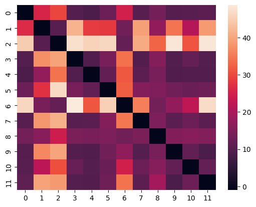
We can see that some of our stations are closer than others, that is, those which have a lower distance show similarities in their time series patterns.
Let's pick 2 that seem different, stations 3 and 6, and see how different they really are:

Seems different enough to be interesting. After all, we're trying to challenge our models here.
So, there are two approaches we can take now: we can either throw all the data at our different models to see how they navigate the different sites or we can train different models on each of our sites and use an ensemble to weight predictions from each model. The promise of deep learning is that we can do the former, so for this article we will try that and do the second in a follow-up.
Training our models
This next section lays out the training of our 5 models using DARTs. The code all lives here but we have most of the code listed out here.
Making some training data
We want to pick some chunk of our data as historical training data, some chunk that we can use as a testing dataset for model fitting, and of course a validation set that we can use once the models have been trained. We need to do a bit of data cleaning in order to make this happen:
#get the variables that we're interested in
ts_df = df[['PM2.5', 'timestamp', 'station', 'wd', 'WSPM', 'TEMP', 'PRES', 'DEWP', 'RAIN', 'O3', 'CO', 'NO2', 'SO2']]

#create an indexed timestamp
d = ts_df.timestamp - pd.to_datetime('2013-03-01 00:00:00')

delta_index = []
for delta in d:
    delta_index.append(int(delta.total_seconds()/3600))

#store our friendly new time stamp
ts_df['ts_ind'] = delta_index

#get just the PM2.5, and ts_ind for the target that we want to predict
target_series = TimeSeries.from_group_dataframe(ts_df[["PM2.5", 'ts_ind', 'station']], group_cols=['station'], time_col='ts_ind')
#now everything other than PM2.5 for the covs
cov_series = TimeSeries.from_group_dataframe(ts_df.drop(["PM2.5",'timestamp'], axis=1), group_cols=['station'], time_col='ts_ind')

# Training is a little complex because some models use historical values, and some don't
# 80% for historical data, 10% for future values, 10% held back to test
future_split_point = int(len(cov_series[0]) * 0.8)
val_split_point = int(len(cov_series[0]) * 0.9)

# since some of our models use past/future and others don't we need to get a little funky here.
# also, we need to make a list of time series instances, one for each station, so we do that here
past_target_series = []
future_target_series = []
test_target_series = []

# we want to match what we had last time in trainig, test hasn't been seen by any model so that's good
for ts in target_series:
    past_target_series.append(ts.slice(0, future_split_point)) #up to our 'present'
    future_target_series.append(ts.slice(0, val_split_point)) #up to our testing
    test_target_series.append(ts.slice(future_split_point, len(ts))) #hold out for testing

#now we do the same with our covariates
past_cov_series = []
future_cov_series = []
test_cov_series = []

# we'll use some of the past series, future series, and test series for our forecasts
for ts in cov_series:
    past_cov_series.append(ts.slice(0, future_split_point)) #up to our 'present'
    future_cov_series.append(ts.slice(0, val_split_point)) #up to our testing
    test_cov_series.append(ts.slice(val_split_point, len(ts))) #hold out for testing


#TCN doesn't use static covariates so we just have the station ID as covars in the time series
non_static_cov = []

for i in range(0, len(cov_series)):
    temp_series = TimeSeries.from_series(pd.DataFrame({'station':[i] * len(cov_series[i])}))
    non_static_cov.append(concatenate([cov_series[i], temp_series], axis=1))
Training Temporal Fusion Transformer
As this name might suggest, a TFT is an transformer-based model that has a self-attention mechanism to capture the complex relationships and dynamics across multiple time sequences. This uses historical target values in a look-back window, optional historical data and optional static covariates that allow you to encode categorical variables as well. This type of architecture is fantastically suited to the sort of problem that we're modeling here. Let's get to training:
from darts.models import TFTModel

early_stop = EarlyStopping(
    monitor="train_loss",
    patience=5,
    min_delta=0.05,
    mode='min',
)

model = TFTModel(
    input_chunk_length=6,
    output_chunk_length=6,
    n_epochs=20,
    pl_trainer_kwargs={
                    "accelerator": "gpu",
                    "devices": [0],
                    "callbacks": [early_stop]
                  }
)

# future_covariates are mandatory for `TFTModel`
model.fit(past_target_series,
          past_covariates=cov_series,
          future_covariates=cov_series,
          val_series=future_target_series,
          val_future_covariates=future_cov_series,
          val_past_covariates=cov_series)
Training Temporal Convolutional Network
A Temporal Convolutional Network is the same sort of convolutional network that you've probably heard of for working with images, but with the kernel modified to use time periods from the training time series. Typically the TCN consists of dilated 1D convolutional layers which models the values in the time series as causal relationships.
from darts.models import TCNModel
from darts.dataprocessing.transformers import Scaler
from darts.utils.likelihood_models import QuantileRegression

from pytorch_lightning.callbacks.early_stopping import EarlyStopping

early_stop = EarlyStopping(
    monitor="train_loss",
    patience=5,
    min_delta=0.001,
    mode='min',
)

model = TCNModel(input_chunk_length=128,
                 output_chunk_length=6,
                 dropout=0.01,
                 pl_trainer_kwargs={
                    "accelerator": "gpu",
                    "devices": [0],
                    "callbacks": [early_stop]
                  })

model.fit(past_target_series, past_covariates=non_static_cov, val_series=future_target_series, val_past_covariates=non_static_cov, epochs=40)
Training NBEATS
The term basis expansion, the BE in NBEATs, is at the heart of this approach. NBEATs consists of multiple stacks, each of which consists of multiple blocks. The first block will look at a small part of the time series and create a prediction. The residuals of that prediction are passed to the following block to create its own prediction based on the residuals. This process is repeated until an accurate prediction is captured. The longer the period of time that the model is trying to predict, the more stacks the model will contain.
from darts.models import NBEATSModel

model_nbeats = NBEATSModel(
    input_chunk_length=30,
    output_chunk_length=7,
    generic_architecture=False,
    num_blocks=3,
    num_layers=4,
    layer_widths=512,
    n_epochs=100,
    nr_epochs_val_period=1,
    batch_size=800,
    model_name="nbeats_interpretable_run"
)

model_nbeats.fit(series=past_target_series,
                 past_covariates=past_cov_series,
                 val_series=future_target_series,
                 val_past_covariates=cov_series,
                 epochs=20)
Training NHiTS
NHiTS is an evolution of NBEATs that samples the time series data at multiple time ranges and then uses a MaxPool layer to interpolate between all the different predictions. The process of combining the different predictions for different time ranges is called hierarchical interpolation, hence the name NHiTS. Like NBEATs, the outputs of multiple stacks are combined but unlike NBEATs, each stack outputs a value for a specific frequency or time range rather than time step in the time series.
from darts.models import NHiTSModel

early_stop = EarlyStopping(
    monitor="train_loss",
    patience=5,
    min_delta=0.05,
    mode='min',
)

model_nhits = NHiTSModel(
    input_chunk_length=48,
    output_chunk_length=6,
    num_blocks=3,
    num_layers=4,
    layer_widths=512,
    n_epochs=100,
    nr_epochs_val_period=1,
    batch_size=800,
    pl_trainer_kwargs={
                    "accelerator": "gpu",
                    "devices": [0],
                    "callbacks": [early_stop]
                  })

model_nhits.fit(past_target_series,
                past_covariates=cov_series,
                val_series=future_target_series,
                val_past_covariates=cov_series)
Training DLinear
D-Linear is the "embarrasingly simple" architecture described in the paper above that we kicked this off with. D-Linear decomposes raw data into a trend and seasonal component, using some classic time series modeling statistical techniques. Two single-layer linear networks are then applied to each component and the outputs are summed to get the final prediction. Pretty simple, pretty elegant when it works.
from darts.models import DLinearModel

from darts.metrics.metrics import rmse, mape

model = DLinearModel(
    input_chunk_length=24,
    output_chunk_length=6,
    n_epochs=20,
)
model.fit(past_target_series, past_covariates=past_cov_series, future_covariates=future_cov_series)
Baseline
And finally we have the simplest possible model: a Naive Drift implementation.
from darts.models import NaiveDrift

nd_model = NaiveDrift()
nd_model.fit(past_target_series[0])
If our models don't perform a Naive Drift, we know they're not really doing their job (or that we haven't done them justice).
Evaluating:
For each of these models we'll use the DARTs backtest() method to see how well it can predict each of our 11 sites. The backteset computes error values that the model would have produced when used on (potentially multiple) series. We're not going to let our models retrain at each step because I don't have that many Colab credits and my AWS piggybank is empty, hence retrain=False. We also want to not test on our entire testing set, for the sake of time, so I'm passing start=0.9 to use 90% of the testing time series. The backtest uses each historical forecast to compute error scores which in this case will be RMSE. The calls for each of our models are going to look very similar with a few small differences for the model architectures:
nbeats_backtest = nbeats_model.backtest(series = test_target_series,
                                  past_covariates=cov_series,
                                  retrain=False,
                                  metric=rmse,
                                  start=0.9)
NBEATs doesn't use future covariates, while TFT does. The TCN doesn't use static covariates so we need to pass an array of timeseries with the station ID encoded as a covariate. Aside from that though, things are fairly uniform. If you're curious about the slight differences in calls, check out [the Jupyter notebook]((https://nbviewer.org/github/joshuajnoble/transformers_4_forecasting/blob/main/model_testing.ipynb).
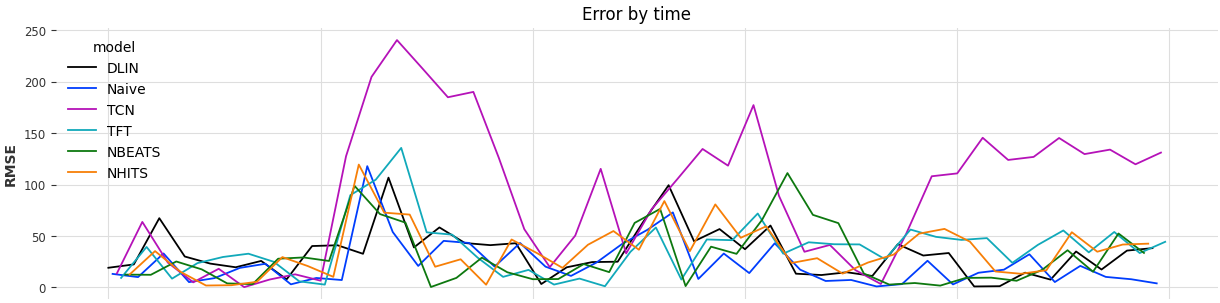
Now the great reveal, how did they do per site?
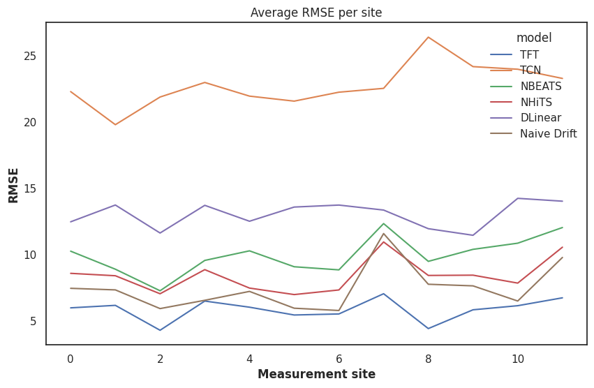
So our Naive Drift is quite good, worryingly good in fact. The only model that outperforms it is our Temporal Fusion Transformer. The Temporal Convolutional Network is treated a bit unfairly by our dataset because it doesn't account for the relationships between multiple covariates and static covariates well enough to keep up with the complexity of our dataset. NHits seems to do fairly well in this shoot-out, likely because the hierarchical nature of the time series windows that it examines can catch the fairly sudden changes in PM2.5.
There's an interesting way that I've found insightful to understand what might be going on when testing forecasting models that we can try out: how different are the errors from the target values? E.g. do the errors themselves track the target value? E.g. is our model failing to catch spikes or anomalies in our data or our covariates?
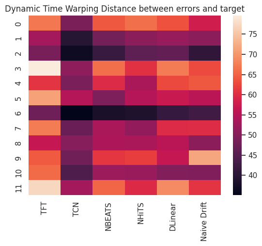
As we might guess, since our TCN model is performing so poorly, the errors that model produces track the actual target values. When PM2.5 goes up, so does our error, when it goes down, so does our error rate. This is a nice way to catch our models that might look good because they just pick the mean over and over again. While that might minimize the RMSE, it's not a sign of a good forecasting model. Our best performing model, the TFT, tends to not have its errors tracking the values. Whatever it's doing wrong, it's doing it wrong in a slightly more interesting way.
Let's open it up to a broader and wider prediction test by expanding the target series that we evaluate against from 10% of the testing set to 50% of the testing set:
start_location = 0.5

naive_backtest_series = nd_model.backtest(test_target_series,
                                          start=start_location,
                                          metric=rmse,
                                          reduction=None)

tft_backtest_series = tftmodel.backtest(series = test_target_series,
                                        past_covariates=cov_series,
                                        future_covariates=test_cov_series,
                                        retrain=False,
                                        metric=rmse,
                                        start=start_location,
                                        num_samples=100,
                                        reduction=None)

# rest of the models backtested below...
Now we can see how our models stack up:
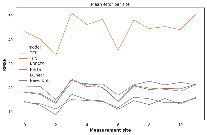
So our TFT still just barely beats the naive drift and the other models still look more or less the same. How much better is our TFT than just a drift?
np.mean(mean_rmse(tft_backtest_series)) - np.mean(mean_rmse(naive_backtest_series))
We get back -0.2236660970731279, not a resounding victory but promising.
Why TFT?
The TFT architecture explicitly recognizes static covariates (like our stations). It encodes them and feeds them into each Gated Residual Network along with selected and encoded variables from a multi-variate time series set. This means that at each step the TFT uses the static covariates in 3 locations: when weighting the variables that most influence the output it's trying to learn with the covariatese, when processing the temporal representations in its Sequence-to-Sequence layer, and when preparing the output of its Gated Residdal Network to pass to the attention mechanism. The weighting of each static covariate varies across each of these steps and across all of the time steps, meaning that our station data can be very important sometimes (e.g. when the wind is blowing in a certain direction with a certain strength) and not at all in others. Because the TFT has a self-attention mechanism rather than purely positional attention mechanism, it can learn that some time steps in the time series are more important than others.
The original paper for the TFT is here, very worth taking a read through.
Digging into the testing
Let's look more closely what's going on in our testing. Here's the PM2.5 values compared to the error rates:
Here's the PM2.5 values compared to the error rates:
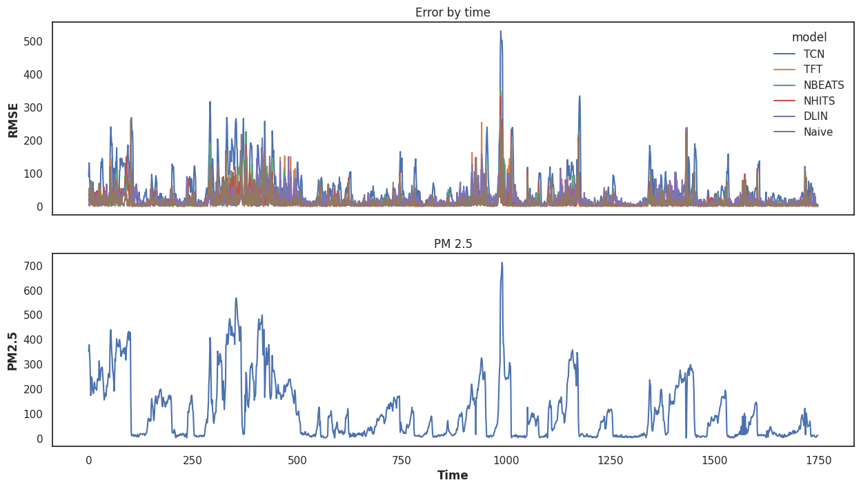
We can see a few interesting things here. First, the data has a lot of challenging features. Second, one of our models truly seem catch the big spikes but some of them recover much more quickly than others. That's part of why the Naive drift does so well: when the PM2.5 drops quickly, it drops along with it quite quickly as well. Other models are still using up too much of the past. That could probably be corrected by shortening the windows that these models use for their inputs.
We could zoom in a little on our models (time indices 900 - 1100) and see what they look like at a particularly spicy time (both for predicting, and for breathing):
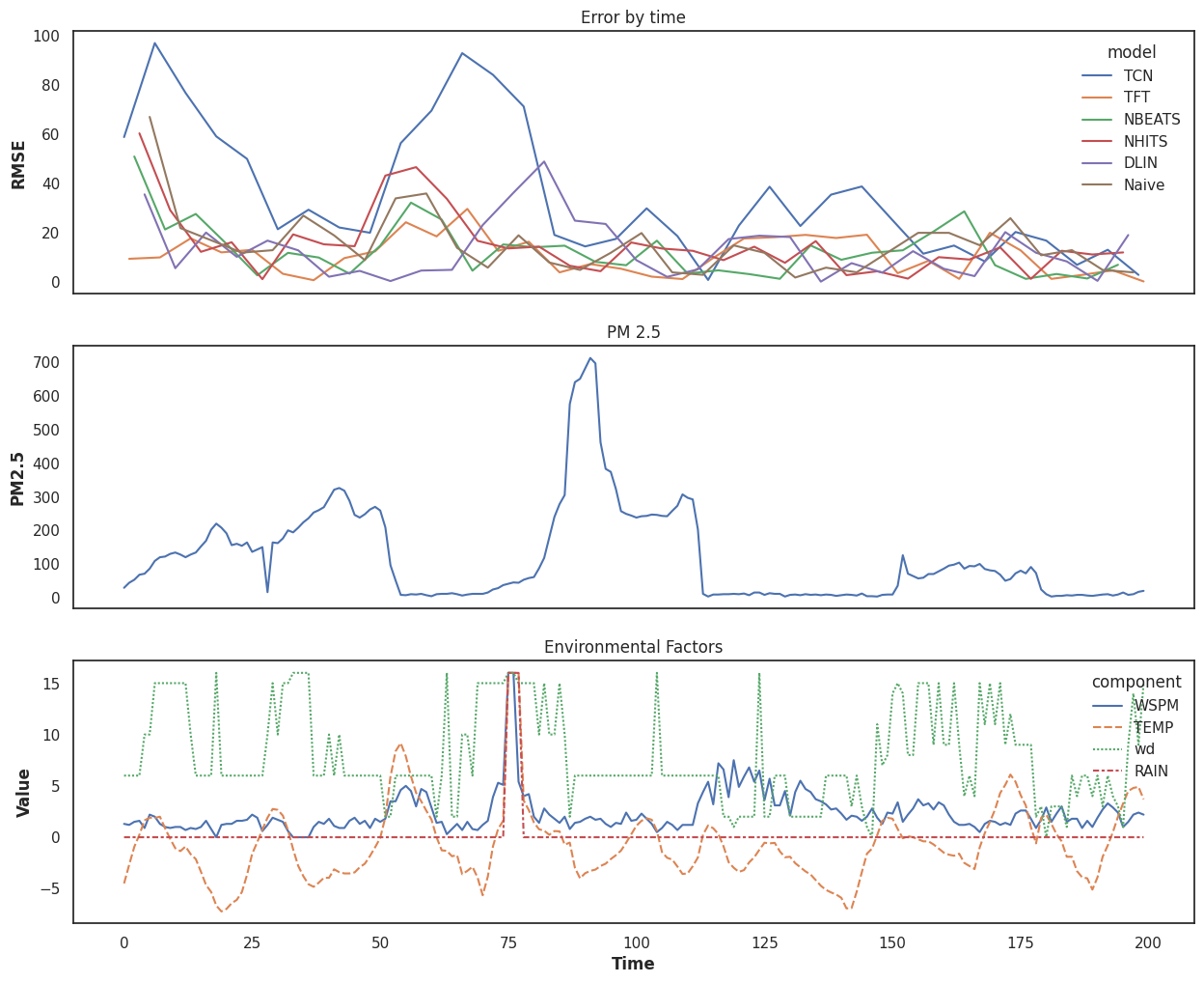
Here we start to get a bit better picture of what might be going on in the middle of our prediction period: the wind blows in some bad air and then dies down. One of our wind directions seems to have a correlation with the PM2.5 when paired with a strong enough wind speed. When the wind shifts to a different direction, after a short lag, the spike dies down. There's also likely something else going on that our data isn't capturing either, but a good forecasting model will capture some of the data while also being flexible to the trends.
We can look at a different time period (time indices 250 - 500) to confirm that this is in fact the case:
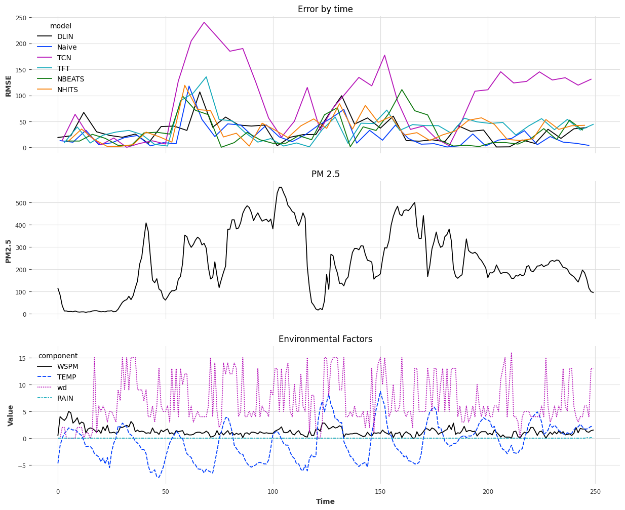
Again, the wind direction and wind speed seem to affect the PM2.5 significantly. Some of our models seem to understand this, others don't but skip actually predicting, and some others seem to handle these relationships moderately well. To confirm that our suspicions are correct, let's normalize all the values for PM2.5, windspeed, and direction and then plot it:
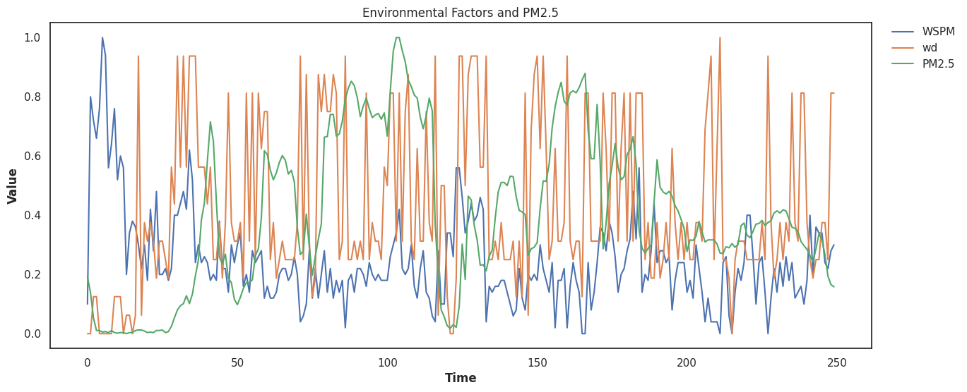
Looks like we have some strong correlations that our models (hopefully) can pick up on.
Wrap Up
The Temporal Fusion Transformer seems to be our winner by a nose over the Naive Drift. That may be disappointing but we're using really challenging data that has significant spikes in it and any model that out-performs a baseline drift is a significant win in my book. Are Transformers really that bad at predicting? Well with this dataset, compared to D-Linear, no, they don't seem to be. Is bigger always better? Not necessarily, but the TFT is one of the more complex model architectures out there. However, throwing more covariates at it likely isn't going to help. We saw that the windspeed and wind-direction were likely the strongest correlations (with a lag) to the PM2.5, so one could take a guess that pulling out just that data might give us slightly better predictive power in our models.
There are some strategies that we probably should use to deal with this and I'm going to keep playing with this data and do another short little article on this soon.